Wherefore BI?
To be frank, an
organization that merely collects and manages its data, and perhaps
reviews that data semi-regularly through basic and ad hoc reports, is
losing out almost completely on the strategic value and the information
that the data holds. Moreover, taking advantage of the basic features of
Analysis Services isn’t that hard, and the concepts aren’t all that
difficult for relational database experts to grasp.
If you look carefully at the
entire suite of features and components in SQL Server 2005, you’ll find
that the biggest advances have come from the BI side. Don’t get us
wrong: New relational database features such as the Service Broker,
native XML support, and the SQL CLR programming model are important in
their own right. But their importance must be understood in the context
of incremental change in a relational database engine that was already mature, sophisticated, scalable, and well understood by the market.
The
advances in Analysis Services, meanwhile, are much more
ground-breaking. The release of SQL Server 2005 Analysis Services marks
the product’s crossover into mainstream ease of use, programmability,
interoperability, and integration with the rest of SQL Server and its
toolset.
We believe
strongly that understanding Analysis Services is totally within reach
for anyone proficient in the relational side of SQL Server. Our goal is
to provide coverage of Analysis Services that is approachable,
practical, and fun.
OLAP 101
Let’s begin our
exploration of Analysis Services with a “quick hit” introduction to
OLAP. You’ll learn the fundamentals of OLAP, including
general OLAP concepts and the basics of how to build, maintain, and
query OLAP cubes in Microsoft SQL Server 2005. Specifically, we’ll cover
the following topics:
Definitions of several terms, including cubes, measures, dimensions, attributes, hierarchies, levels, members, and axes
Data warehousing concepts and the motivation behind so-called star and snowflake schemas
The
basics of Visual Studio Analysis Services projects, such as data
sources, data source views, the cube and dimension designers, and
various wizards
Querying cubes in the cube designer’s Browser tab
As we just
mentioned, SQL Server first brought OLAP functionality to us in version 7
with OLAP Services, a product that was essentially separate from,
though bundled with, SQL Server proper. SQL Server 2000 Analysis
Services included better OLAP functionality and new data mining
capabilities but offered only slightly better integration with the SQL
Server relational database. Analysis Services in SQL Server 2005 brings
huge improvements in functionality over its predecessor, much better
integration into the product, an architectural “rethink,” and impressive
ease-of-use features.
OLAP, which is an acronym for the rather vague moniker “online analytical processing,”
can be thought of as database technology optimized for drill-down
analysis. That’s it! Forget all the confusing explanations you may have
heard—there’s really no magic here, and it need not be confusing. OLAP
allows users to perform drill-down queries incredibly quickly and does
so in two ways:
OLAP cubes store
so much data that in many cases, both the high-level roll-ups and
midlevel and low-level drilled-down figures needed for any given query
are already calculated and need only be output.
Even
calculations that need to be done on the fly can be performed quickly
because an OLAP engine is optimized for this task and doesn’t need to
concern itself with the complex tasks of a relational database, such as
managing indexes, performing joins, or (except in specific
circumstances) dealing with updates and concurrency. OLAP cubes
essentially contain data at the lowest drilled-down levels, calculate
some or all of the higher-level aggregations when a cube is built, and
calculate the others at query time by aggregating the lower-level
numbers already in the cube.
The result is a
technology that lets users do an incredible amount of exploration
through their data, allowing them to entertain a number of ad hoc,
what-if scenarios without worrying about the time and resources it would
take a relational engine to satisfy the same queries. If users
don’t have to be “afraid” to ask their questions, they’ll ask a lot
more of them, gain useful insight into their data, make better business
decisions, and get a much higher return on investment on the relational
systems that supply the cubes’ data in the first place.
OLAP Vocabulary
A cube, which is the OLAP equivalent of a table in a relational database, consists of measures, which are the numeric data that users will analyze (for example, sales amount), and dimensions,
which are the categories that the measures will be drilled down by (for
example, Time, Geography, Shipper, or Promotion). Dimensions can be
hierarchical. For example, a Geography dimension would likely be
hierarchical and might consist of country, state/province, city, and
postal code levels. The individual countries, states, and so on are called the members
of their respective levels. Such a scheme allows users to break down
sales by country, then drill down on a specific country (good to do if
that country’s sales are particularly high or low), then on a specific
state or province within that country, then on specific cities in that
state or province, and then even on postal codes in one or more of those
cities. (This would allow a user to pinpoint quickly why a particular
country’s sales are so high or low.)
This all seems
elementary and unsophisticated, doesn’t it? Are you disillusioned? Don’t
be. Let’s up the ante a bit: Imagine a spreadsheet where the columns
contain the set of countries in which a company operates, the rows
contain each of the four quarters of the last fiscal year, and each cell
contains a sales figure for each corresponding combination of country
and fiscal quarter. Imagine further that users can drill down on any
quarter (to reveal the three months within it) and/or any country to
reveal the sales numbers for those cross-sections of the cube. Imagine
that the spreadsheet is replicated numerous times, once for each
salesperson’s sales data, where each of these spreadsheets offers the
same drill-down capabilities, returning the specific results implied by
the drill-down, quickly and easily.
This entire set of
spreadsheets can be returned by an OLAP engine with one fairly simple
query. Still not impressed? Imagine each of the sales numbers in each
spreadsheet appearing next to the corresponding year-ago figure and
that, even with this enhancement, the whole interactive drill-down
report can still
be produced with a single query. Hopefully, we’ve caught your attention
and have given you some insight into the power and business value of
OLAP.
Dimensions, Axes, Stars, and Snowflakes
Let’s go back to some
definitions. Because OLAP cubes and even OLAP query result sets can
contain data along multiple physical dimensions, not just rows and
columns, the term multidimensional
is often used to refer to OLAP databases. In fact, the language you use
to query SQL Server OLAP cubes is called MDX (which stands for
“multidimensional expression language”). The object models used to write
OLAP applications are called ADO MD (the COMbased object model) and ADO
MD.NET (its .NET managed equivalent); in both cases, the MD stands for multidimensional.
Thinking tangibly about multidimensional data can be visually and
logically challenging. Be prepared for this so that you are not
discouraged along the way; meanwhile, we’ll do our best to get you
through it.
OLAP
cubes are created from a collection of special tables in a relational
database: fact tables and dimension tables. To illustrate what’s in each
of these, imagine a simple cube containing unit sales, total sales, and
discount as its only measures and supplier and geography as its only
dimensions. Imagine that the supplier dimension is flat, that is,
nonhierarchical, and that the geography dimension is hierarchical, with
its lowest level being postal code. The fact table then needs to contain
the sales data for products from each supplier in each postal code.
Each row contains a postal code in one column, a key for a supplier in a
second column, and the corresponding measures data in additional
columns. Each possible combination of postal code and supplier
corresponds to a separate row in the fact table (except for postal codes
where specific shippers were not responsible for any sales).
We also need dimension
tables. Let’s start with a dimension table for the supplier. This is
simply a lookup table containing the supplier key and name in separate
columns. You can see how joining the fact table to this table on
supplier ID will allow us to get the shipper’s name for each
shipper/postal code fact data row.
Because
geography is hierarchical, the relationship between the fact table and
the dimension table is more complex. The geography dimension’s
information can be captured in a single, denormalized table that
corresponds to each unique postal code with a city, state/province, and
country, or you can have separate, normalized lookup tables for each
level in the hierarchy. (You can also have a combination of
semi-denormalized tables, each combining a couple of hierarchical
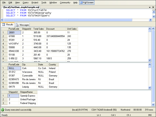
levels.) See Figure 1
for a sample representation of the data in the fact table and the two
denormalized dimension tables. Notice that the fact table contains only
measure data and foreign keys to the lowest level of each of the two
dimensions.
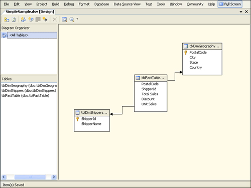
Once
the cube is built, the normalized or denormalized basis of its
dimensions matter very little, so your choice at cube design time is
essentially one of convenience. In the case of fully denormalized
dimension tables, the schema ends up consisting of a fact table in the
center with “spokes” branching out to each dimension table, as shown in Figure 2. The geometry of this type of schema suggests a star, so it is often referred to as a star schema.
Dimensions that involve multiple tables somewhat weaken the star-like
analogy because the spokes have multiple nodes. Dimensions with multiple
tables are therefore more commonly referred to as having a snowflake schema (a snowflake essentially resembling a more geometrically complex version of a star).
Typically,
databases with star/snowflake schemas are created by taking normalized
databases and running scripts, stored procedures, or ETL (extract,
transform, and load) processes on them to create the transformed fact
tables and dimension tables. These tables can be created in a new
standalone database, and they in effect form the basis of a data
warehouse. As such, they can serve as excellent data sources for running
relational reports as well. Given that these tables have some degree of
denormalization, they are easy to create reports against, and because
they’re in a separate database, or at least exist as separate tables in
the main database, allowing users to run reports from them poses no
strain on the production online transaction processing (OLTP) tables. If
you find the physical transformation of the data inconvenient, remember
that fact and also that dimension “tables” can, in fact, be views.